Selfishness and eradication of disease

Consider a population at risk of an infectious disease, where individuals recover but will eventually become susceptible again. The population is divided into two groups. The first group decides to use some health intervention, which comes to the benefit of preventing infections but also to some nuisance cost. The second group will not use the health intervention, they are at higher risk of infection, but do not bear the nuisance cost.

If we let the dynamics of disease transmission and individual preference co-evolve, what happens on the long run at the population level? Will the disease persist? Or will the parasite disappear from the population?

THE EPIDEMIOLOGICAL MODEL

We consider a population divided into two groups: Users ($U$) and Non-users ($N$). Each group is further divided into Susceptible ($S$) and Infectious ($I$) compartments. The total population is normalized to $1$ and remains constant: $S_U + I_U + S_N + I_N = 1$.

The transmission is governed by the force of infection $\lambda = (1-\sigma)\beta (I_U + I_N)$, where $\beta$ is the transmission rate and $\sigma$ is the protective efficacy of the bednet ($0 \leq \sigma \leq 1$). The recovery rate is $\gamma$. The system of differential equations is:

\[\begin{align} \frac{dS_U}{dt} &= -(1-\sigma) \beta S_U (I_U + I_N) + \gamma I_U \\ \frac{dI_U}{dt} &= (1-\sigma) \beta S_U (I_U + I_N) - \gamma I_U \\ \frac{dS_N}{dt} &= -\beta S_N (I_U + I_N) + \gamma I_N \\ \frac{dI_N}{dt} &= \beta S_N (I_U + I_N) - \gamma I_N \end{align}\]

Let $x$ denote the frequency of intervention users in the population ($x = S_U + I_U$). Thus setting $S_U=x-I_U$ and $S_V=(1-x)-I_V$, the system can be reduced to $\begin{align} \frac{dI_U}{dt} &= (1-\sigma) \beta (x-I_U) (I_U + I_N) - \gamma I_U \\ \frac{dI_N}{dt} &= \beta (1-x-I_N) (I_U + I_N) - \gamma I_N \end{align}$

Using the next generation matrix approach to calculate the basic reproduction number $R_0$:

\[F = \begin{pmatrix} (1-\sigma)\beta x & (1-\sigma)\beta x \\ \beta(1-x) & \beta(1-x) \end{pmatrix}, \quad V = \begin{pmatrix} \gamma & 0 \\ 0 & \gamma \end{pmatrix}\]

The Next-Generation Matrix is $K = FV^{-1}$:

\[K = \begin{pmatrix} \frac{(1-\sigma)\beta x}{\gamma} & \frac{(1-\sigma)\beta x}{\gamma} \\ \frac{\beta(1-x)}{\gamma} & \frac{\beta(1-x)}{\gamma} \end{pmatrix}\]

$R_0$ is the spectral radius (the largest eigenvalue) of matrix $K$ and reads $R_0(x,\sigma) = \frac{(1-\sigma)\beta x}{\gamma} + \frac{\beta(1-x)}{\gamma}$. This gives $R_0(x,\sigma) = \frac{\beta}{\gamma} ( (1-\sigma)x + (1-x) )=\frac{\beta}{\gamma} ( 1-\sigma x )$

The disease dies out if $R_0(x,\sigma)<1 \Leftrightarrow x > \frac{1}{\sigma} (1 - \frac{\gamma}{\beta})$.

We call $x^e=\frac{1}{\sigma} (1 - \frac{\gamma}{\beta})$ the user frequency elimination threshold.

REPLICATOR DYNAMICS FOR INTERVENTION USAGE

The decision to use an intervention is modeled as a game. Like in a lottery, each host can play two different strategies against the bank, which is here the pool of infectious hosts in the population. If the host decides to not use the intervention, she will suffer from the potential consequences of an infection at cost $C_I>0$. If the host decides to play as a user, he will suffer a little less from the consequences of an infection, but incur the nuisance cost $C_N\geq 0$ of putting and maintaining the net every day. For both strategies we can write the individual payoff as negative values of the cost:

$f_U = -C_N - (1-\sigma) \beta I C_I$$

\[f_N = -\beta I C_I\]

The population payoff is

\[\bar{f}(x)= xf_U+ (1-x)f_N\]

We assume that individuals do not interact with other individuals’ strategies to determine their own cost, like it would be in a card game. To play against the entire infectious population is actually in accordance with the mass-action principle for disease transmission.

The evolution of user frequency $x$ satisfies the replicator equation:

\[\begin{equation} \dot{x} = x (f_U - \bar{f}(x)) \end{equation}\]

In our case, this equation simplifies to

\[\begin{equation} \dot{x} = x ((1-x) f_U - (1-x) f_N) = x(1-x)(f_U-f_N) \end{equation}\]

also known as logistic growth equation.

The intervention user behavior dynamics is governed by

\[\begin{equation} \dot{x} = x(1-x) ( \sigma\beta I C_I - C_N ) \end{equation}\]

We distinguish:

Adoption: $x$ increases if $\beta I > \frac{C_N}{C_I \sigma}$. The risk-reduction benefit outweighs the nuisance cost.
Abandonment: $x$ decreases if $\beta I < \frac{C_N}{C_I \sigma}$. The nuisance cost is perceived as greater than the expected cost of infection.
Evolutionary Stability: A mixed equilibrium exists when $\beta I = \frac{C_N}{C_I \sigma}$.

EQUILIBRIUM FOR INFECTIOUS DISEASE DYNAMICS

To find the endemic equilibrium of the reduced system $\begin{align} \frac{dI_U}{dt} &= (1-\sigma) \beta (x-I_U) (I_U + I_N) - \gamma I_U \\ \frac{dI_N}{dt} &= \beta (1-x-I_N) (I_U + I_N) - \gamma I_N \end{align}$ We need to consider the case $R_0(x,\sigma)>1$ and solve $dI_U/dt = 0$ and $dI_N/dt = 0$.

Let $I = I_U + I_N$ be the total prevalence.

Then $I_U^* = \frac{(1-\sigma) \beta x I}{(1-\sigma) \beta I + \gamma}$ and $I_N^* = \frac{\beta (1-x) I}{\beta I + \gamma}.$

Since $I = I_U + I_N$, we sum the two equations: $I =( \frac{(1-\sigma) \beta x}{(1-\sigma) \beta I + \gamma} + \frac{\beta (1-x)}{\beta I + \gamma} ) I$

If $I > 0$, we can divide both sides by $I$:

\[1 = \frac{(1-\sigma) \beta x}{(1-\sigma) \beta I + \gamma} + \frac{\beta (1-x)}{\beta I + \gamma}\]

This is a quadratic equation in $I$: $\beta^2 (1-\sigma) I^2 + \beta ( \gamma(2-\sigma) - \beta(1 - \sigma ) ) I + \gamma^2 ( 1 - R_0(x,\sigma) ) = 0$

The positive root of this quadratic gives the unique endemic equilibrium level when $R_0(x,\sigma ) > 1$:

$I^* = \frac{-B + \sqrt{B^2 - 4AC}}{2A}$ for $A = \beta^2 (1-\sigma)$, $B = \beta \gamma (2-\sigma) - \beta^2(1 - \sigma )$ and $C = \gamma^2 (1 - R_0(x,\sigma))$.

EQUILIBRIUM FOR THE COUPLED DISEASE-REPLICATOR DYNAMICS

We can also solve the quadratic equation in $I$ for $x$ to obtain the user frequency at the endemic equilibrium. From the replicator equation we know that the user frequency is at equilibrium if the payoffs for users and non-users are equal: $f_U = f_N$ which amounts to mainting a specific prevalence:

$\bar{I} = \frac{C_N}{\sigma\beta C_I }$ in the population.

Solving the quadratic equation for $x$ by using the expression for $R_0(x,\sigma)$ yields

\[\bar{x} = \frac{1}{\sigma}(1-\frac{\gamma}{\beta})- \frac{(\gamma(2-\sigma) - \beta(1 - \sigma ))}{\gamma \sigma} \bar{I}- \frac{\beta (1-\sigma) }{\gamma \sigma}\bar{I}^2\]

The strategy $\bar{x}$ is an evolutionary stable strategy for the case where the disease will persist and eventually reach an endemic equilbrium $\bar{I}$. The coupled disease-replicator dynamics is at equilibrium $(\bar{I},\bar{x})$, which depends on both disease or efficacy parameters $\beta, \gamma, \sigma$ and net usage behavior parameters $C_N$ and $C_I$.

ELIMINATION THRESHOLD AND ERADICATION GAP

Let us recall the elimination threshold of user frequency $x^e = \frac{1}{\sigma} \left( 1 - \frac{\gamma}{\beta} \right)$

It follows that $\begin{equation}\bar{x} = x^e + \frac{\beta(1-\sigma) - \gamma(2-\sigma)}{\gamma \sigma} \bar{I} - \frac{\beta (1-\sigma)}{\gamma \sigma} \bar{I}^2\end{equation}$

The difference $\Delta=x^e-\bar{x}$ is called the eradication gap.

\[\Delta = \frac{\bar{I}}{\sigma} (2 - \sigma - \frac{\beta}{\gamma}(1-\sigma) + \frac{\beta}{\gamma}(1-\sigma)\bar{I})>\frac{\bar{I}}{\sigma} (2 - \sigma - \frac{\beta}{\gamma}(1-\sigma))= \frac{C_N}{\beta C_I }(1 + (1-\sigma)(1-\frac{\beta}{\gamma}))\]

As the nuisance cost $C_N$ increases, the gap is widening. Equality between the elimination threshold and the evolutionary stable strategy can only hold if the nuisance cost is $C_N=0$. This means that as long as interventions are effective and have a non-zero nuisance cost, non-users will free-ride at the expense of users and jeopardize the eradication.

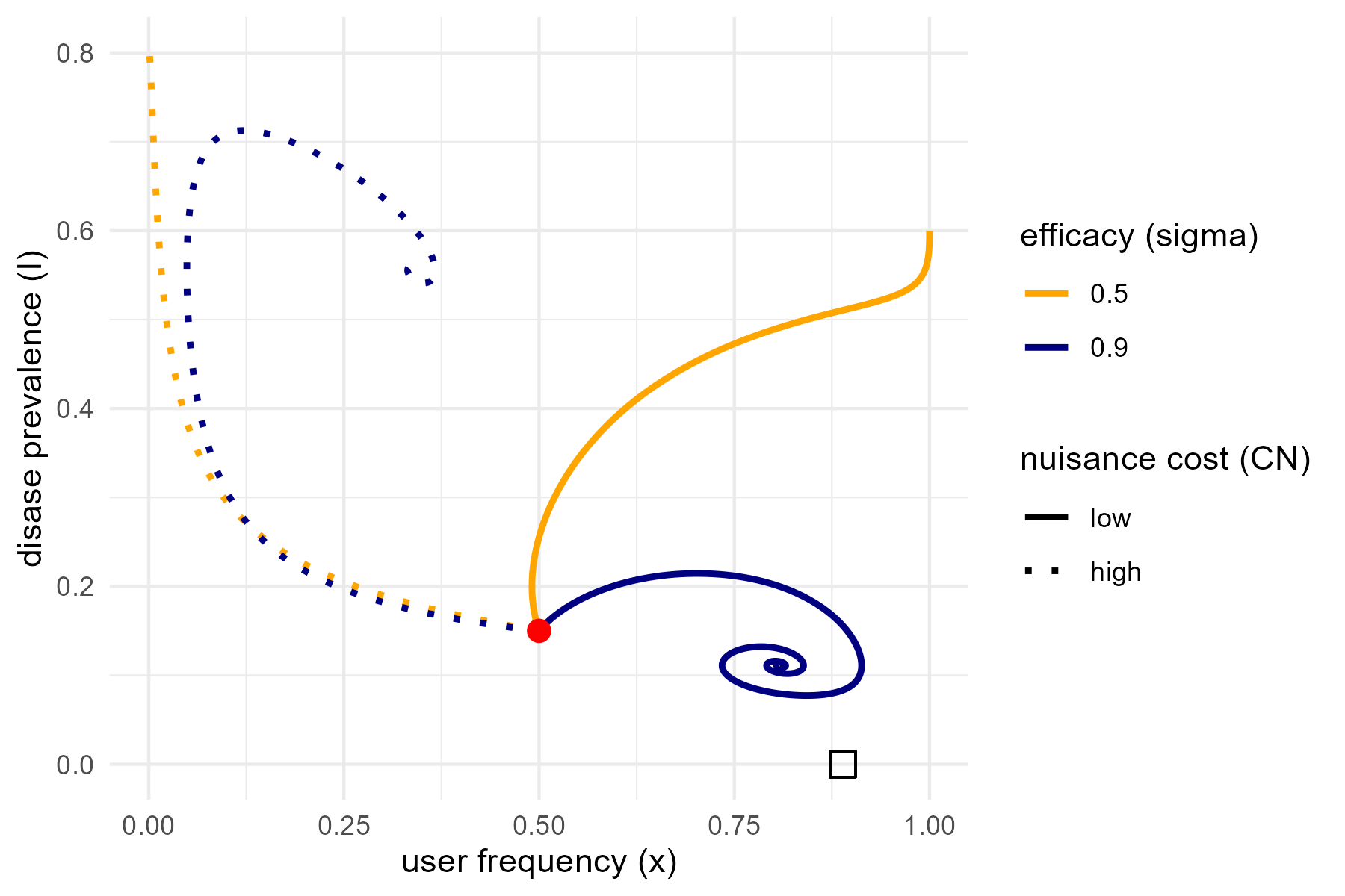
The figure depicts the phase diagram of the coupled model of user frequency and disease prevalence for two different choices of efficacy and nuisance. The dynamical systems starts at the red point. At low efficacy and low nuisance, everyone will end up using the intervention and the equilibrium is at high prevalence. Increasing nuisance at low efficacy will result in no users and the entire population infected. Increasing efficacy but having low nuisance creates an opportunity for free-riders, resulting in lower endemic equilibrium and intermediate user frequency. Again, increasing nuisance in the high efficacy case will deter users and result in a high endemic equilibrium. The elimination threshold for $\sigma=0.9$ is located at the cube on the x-axis, at zero prevalence.