Disease transmission models going neural

Let’s start with an elementary, but yet insightful equation system commonly known as the SIS disease transmission model. Full stop. Let’s start from somewhere else.

The fact that biological entitities such as viruses, bacteria and fungi have durably colonized the human body sets the stage for a life-long antagonistic relationship between them and us - the parasites and the hosts. But not only this unfriendly relationship sets them apart from each other, these best enemies live on distinct spatial and temporal scales. Viruses are sized in the micrometers and can only be observed via electronic microscopy, and one virus can produce offspring in the tens of thousands within hours or days. On the other hand, multicellular tissue heaps known as humans are sized in meters, and it takes decades for them to reproduce, if at all. The action starts when parasites enter human cells, mainly by tricking their surface proteins and making it into the cellular reproduction machinery. Parasites exploit the host cell for their own metabolism or reproduction. Eventually the host cell will disintegrate, parasite offspring is released into the cellular environment to find its next victim. But one host is not enough. Insatiable as they are, the parasites need to transmit in order to continue living, as their fate is bound to the host. In order to enter into new hosts, parasites undergo continuous selection, their genetic makeup changes randomly as they replicate. Full stop.

For microbiologists, this description of a parasite’s lifecycle might sound like an overly simplified vulgarisation, yet it is a physicist’s nightmare: biochemical entities interacting at multiple scales. From the medical perspective, we are dealing with discrete, host-centric events: life, death, infection, symptoms, recovery. This is where disease transmission models start from. Disregarding the complexities of biochemical interactions that allow the parasites to enter host cells and ignoring the evolutionary ecology of parasite population dynamics, they assign each host to a compartment. Like in the old days, when train coachs were divided into compartments, one could comfortably talk, eat and smoke (sic!) in the compartment, granted that all individuals in the compartment would be alike. In the same way, all hosts that share attributes such as susceptible (to infection), infectious (to other hosts) or recovered (from infection) are put into their respective compartment. A rather ad-hoc set of rules defines how hosts can change between compartments, e.g. an infectious host might recover after some time, in the same way as people move from the non-smoking to the smoking compartment on the train. Disease transmission models track the size of the compartments over time. Differential equation techniques of the ordinary, stochastic, delay or partial kind have been invoked to produce model solution curves to be aligned with epidemiological observations.

Let’s start again with an elementary system of differential equations, which models the temporal evoluation of only two compartments, susceptible (S) and infectious hosts (I). Let’s denote the total population size with $N=S+I$ and assume that $N$ remains constant. We posit two ad-hoc rules of transitioning between compartments.

First, for each susceptible host, the probability of finding an infectious host in the population is $\tfrac{I}{N}$, and since there are $S$ susceptible hosts, we would have on average $\beta S \tfrac{I}{N}$ susceptible hosts moving to the (I) compartment. The parameter $\beta>0$ encapsulates all the biochemical and eco-evolutionary complexities that we were so proud to be ignorant of.

Second, infectious hosts might also recover from infection and move to the susceptible compartment with rate $\gamma$, and we would end up with $\gamma I$ hosts on overage moving from the (I) compartment to the (S) compartment.

Differential equations bear their name from the physical principle of motion. In order to describe the trajectory of an object, we only need to know its initial position and its velocity. From the point of view of measurement, velocity should be seen as change of position between two consecutive time points. Mathematicians would paraphrase this measurement of change as difference quotient, and as the distance between consecutive time points gets very small, they would refer to the change as differential quotient or short differential. In its simplest form, this differential depends only on the position itself. So, differential equation, here you are! On your left-hand side, we put the differential to measure infinitesimal change in position, on your right-hand side we put some function of position and other things to quantify the strength of change. Mathematicians are fond of definitions, and even have a name for your right-hand side: they call it a vector field.

Our SIS system reads: $\begin{aligned} \label{eq:sis} \frac{dS}{dt} &= -\beta S \tfrac{I}{N} + \gamma I \\ \frac{dI}{dt} &= \beta S \tfrac{I}{N} - \gamma I \end{aligned}$

Under the assumptions of constant population size we set $S=N-I$ and the SIS system simplifies to a single equation: \begin{equation} \label{eq:sis_simple} \frac{dI}{dt} = \beta (N-I) \tfrac{I}{N} - \gamma I = (\beta - \gamma)I- \tfrac{\beta}{N}I^2 \end{equation}

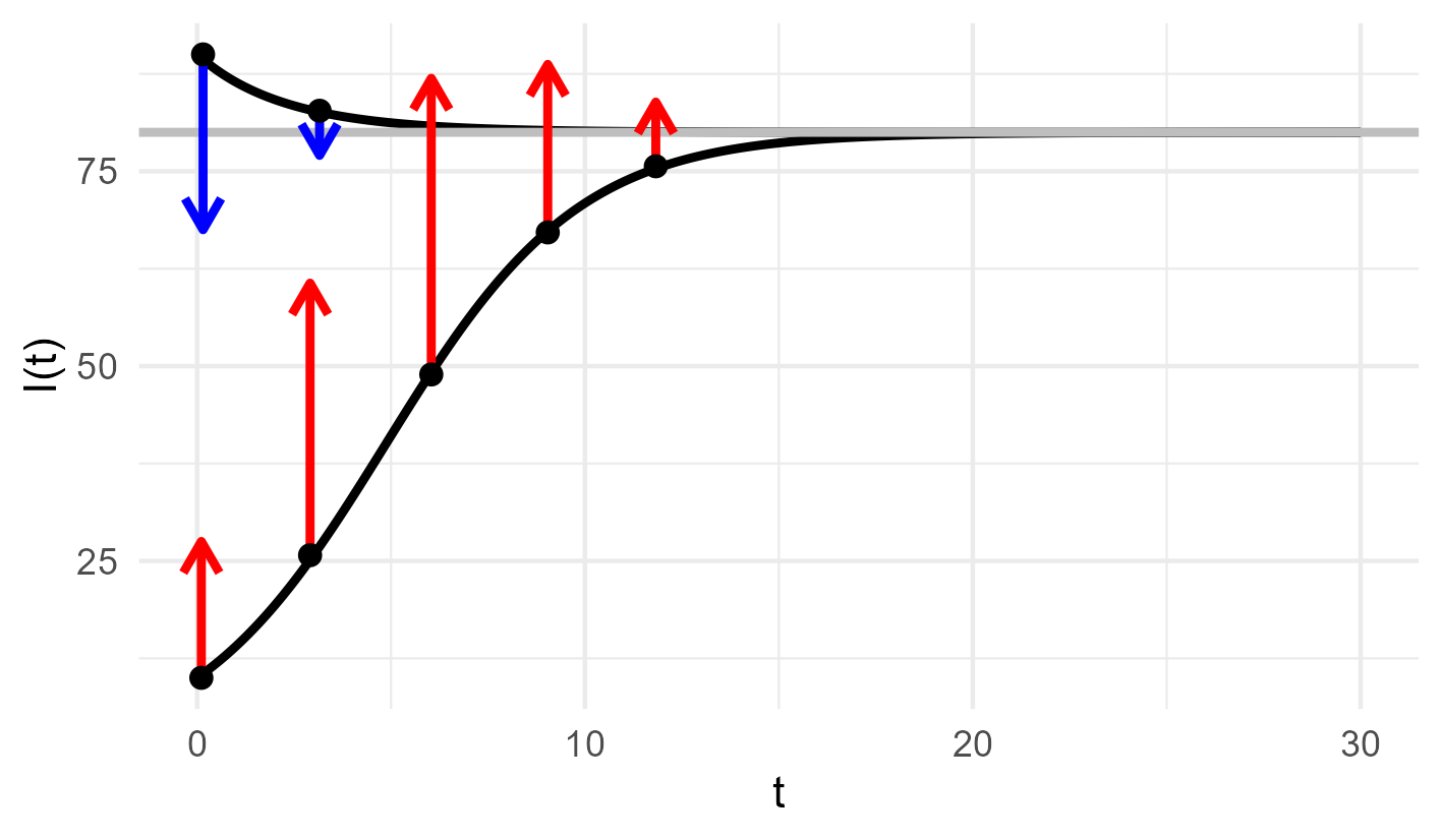
Our differential is $\frac{dI}{dt}$ and the vector field reads $f(x)=(\beta - \gamma) x - \tfrac{\beta}{N}x^2$. The linear part $x\mapsto (\beta - \gamma)x$ of the vector field describes how the balance between new infections and recovery relates to the growth of (I), especially in the beginning. If $\beta - \gamma<0$, negative growth will push eventually the system to the state $I=0$, the so-called disease-free equilibrium. If $\beta - \gamma>0$, the non-linear part $x\mapsto -\tfrac{\beta}{N}x^2$ of the vector field helps to keep the system in place: there cannot be more than $N$ host! If $I$ is close to $N$, the $\beta N$ terms cancel out and $x\mapsto -\gamma x$ will push the sytem to lower values of $I$, it will eventually reach $I=N\tfrac{\beta - \gamma}{\beta}=N\left(1-\tfrac{\gamma}{\beta}\right)$, the so-called endemic equilibrium.

Let’s come back to the rather opaque parameter $\beta>0$. We admitted that we packed all the biochemical and eco-evolutionary complexities that modulate the infectiousness of the parasite into this parameter. Let’s put in some effort and make it at least time-dependent. To keep things simple, let us assume that $t\mapsto \beta(t)$ is non-negative and periodic with fixed amplitude $\theta_1$>0 and period $\theta_2>0$: \begin{equation} \beta\equiv\beta(t)\equiv\beta(t,\theta_1,\theta_2)=\theta_1\left( 1+ \sin \tfrac{2\pi t}{\theta_2}\right) \end{equation} Periodicity of $\beta$ makes sense for a parasite such as influenza virus from the point of view of its biochemistry. It is in dry and cold climate during winter that the protecting lipid layer becomes solid-like, the virus persists in the environment. The surface protein so important for cell entry is conserved in its polymer structure, the virus remains infectious. Not to speak of hosts crowding in trains and classrooms during cold season. Packing all the biochemical complexity into a sine function seems like a mathematical leap of faith bound to fail. Let’s put our model to the test of observations.

Coming back from a lengthy field trip to a remote island, your epidemiologist neighbour carries a dataset full of observations in his backpack. After some data cleaning, he gives you the number of infectious hosts recorded at $K$ distinct time points: $\iota(t_1),\dots,\iota(t_K)$. From his anectotal notebook about the disease you calculate the recovery rate $\gamma$. So far, so good. In order to compare this data to model outputs, we define how far the model outputs are away from the data by an error function: \begin{equation} J = \sum_{j=1}^{K} g(I(t_j), \iota(t_j)) \end{equation} To make things easier, we use the error function $g(x,y)=\tfrac{1}{2}|x-y|^2$ and $J$ is called the residual sum of squares. But there is yet another way to look at $J$. It is a functional. A functional is like a function, only that it is defined on a larger, often infinite-dimensional space such as the space of all possible solution curves to our SIS model with parameters $(\theta_1,\theta_2)$. Remember, we keep $\gamma$ fixed since we trust our epidemiologist neighbour, and $\beta$ was defined by the amplitude and the period. The functional $J$ maps the solution curve $I(t)$ to a real number, the error between the model and the observations. The task of parameter inference is to find values for $(\theta_1,\theta_2)$ such that $J$ is minimal.

Lagrangian multiplier Hamiltonian, adjoint; Lagrangian with time-dependent multiplier Pontryagin

\[H(I, \lambda, \beta, \gamma) = L(I, t) + \lambda(t) \left[ (\beta - \gamma)I - \frac{\beta}{N}I^2 \right]\]

\begin{equation} \label{eq:cauchy-schwarz} \left( \sum_{k=1}^n a_k b_k \right)^2 \leq \left( \sum_{k=1}^n a_k^2 \right) \left( \sum_{k=1}^n b_k^2 \right) \end{equation}

and by adding \label{...} inside the equation environment, we can now refer to the equation using \eqref.

Note that MathJax 3 is a major re-write of MathJax that brought a significant improvement to the loading and rendering speed, which is now on par with KaTeX.